Bug report

When a cell/row is selected, its first cell is focused and the sheet is scrolled to show it. If a long sheet is scrolled down/right to edit cells, this scroll top/left is very annoying and user unfriendly.
In these scenarios Excel focuses the topmost/leftmost currently visible cell, avoiding sheet scrolling.

Reproduction of the problem

1. Go to https://demos.telerik.com/kendo-ui/spreadsheet/index
2. Scroll to the bottom row of Spreadsheet's sheet.
3. Click in cell B200 to select it.
4. Click on the header of column C to select the whole column.

NOTE: for rows reproduction select cell AX2, then click on the header of row 2 - sheet is scrolled to the left and cell A2 is focused.

Current behavior

Column C is selected, cell C1 is focused and the sheet is scrolled to top.
The used has to scroll down to the bottom row again to edit data at the bottom of the sheet.

Expected/desired behavior

Column C is selected. The currently visible topmost cell of column C is focused, without scrolling the sheet. Excel works that way

Environment

• Kendo UI version: 2019.2.619
• Browser: all

Bug report

The current client-side export functionality does not preserve the number of columns.

Reproduction of the problem

• Load the following file in the Spreadsheet which contains columns up to "BA".

• Export the file

• Load the file again in the Spreadsheet and notice that the columns are displayed up to "AX" instead of "BA".

Current behavior

Client-side export does not preserve the number of columns greater than "AX".

Expected/desired behavior

Client-side export does not preserve the exact number of columns.

Environment

• Kendo UI version: 2019.2.619
• Browser: [all]

Dear Concerned,

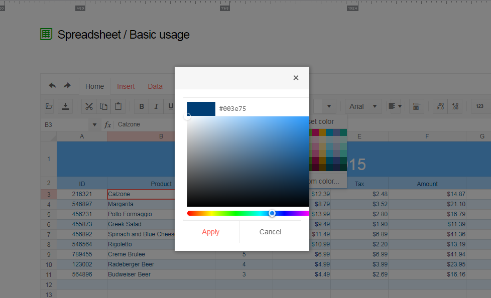
1. Launch https://demos.telerik.com/kendo-ui/spreadsheet/index

2. Click Background or Text Color icon , select custom color

3. See the popup UI , there is boarder and margin issues, boarder is visible on top,left & bottom side but not on right side

Dear Concerned,

1. Open https://demos.telerik.com/kendo-ui/spreadsheet/index

2. Copy from F3:F15

3. Paste as value (ctrl+shift+v) in H3

4. See it pasted only non-empty cells

Empty cells values should be pasted as well as Excel does.

 

Bug report
Spreadsheet SUMIF function returns #NA when Excel returns the correct result. The issue is observed when the criteria range and sum range have different sizes.

Reproduction of the problem
Run the Spreadsheet demo page
Open the attached file
Formula in cell B3 returns #NA!

Current behavior
The formula in cell B3 returns #NA!

Expected/desired behavior
The formula in cell B3 should return the correct value

Environment
Kendo UI version: 2019.3.1023
Browser: [all]

I would like to be able to generate PDF from spreadsheet using HTML template (like http://dojo.telerik.com/Ovegu), so i could specify headers and footers for all PDFs that are created by the user.

The FromJson method of Telerik.Web.Spreadsheet.Workbook doesn't add images when a JSON containing an image blob is passed to it. 

It would be nice if the FromJson method supports images.

Dear Concerned,

1. Open https://demos.telerik.com/kendo-ui/spreadsheet/index

2. Import attached Book21.xlsx file

3. I have first row as frozen pane and columns C, D are hidden

4. Select columns B to E using mouse drag & then right click on selected column , it does not show Unhide option, because on right click it keeps the selection only on column E

It does not work if we keep Freeze Panes.

It would be useful if it is possible to filter between a range of values, like in Excel. For example filter for values that are between 3 and 6.

Bug report

Reproduction of the problem

Dojo example.

Current behavior

The first row is duplicated.

Expected/desired behavior

The first row is not duplicated

Environment

• Kendo UI version: 2019.3.1023
• jQuery version: x.y
• Browser: [all]

Bug report

If an Excel file that contains Shapes is imported in the Spreadsheet, the imported content cannot be exported back to '.xlsx' file. Saving the imported content to Excel throws an error in the console.

Reproduction of the problem

1. Open this demo
2. Import the attached "Download Issue.xlsx" file that has one shape and one Image in the Sheet1.
3. The file import will be successfully executed. The shape from the file is not visible in the Spreadsheet(this is expected behavior as the Spreadsheet component does not support Shapes, so they are ignored during the import process)
4. Export(save) the Spreadsheet content as Excel file

Current behavior

Exporting the Spreadsheet content throws an error in the console:

Expected/desired behavior

The Spreadsheet content should be exported to Excel file that doesn't contain the shapes from the imported file

Environment

• Kendo UI version: 2019.3.1023
• jQuery version: x.y
• Browser: [all]

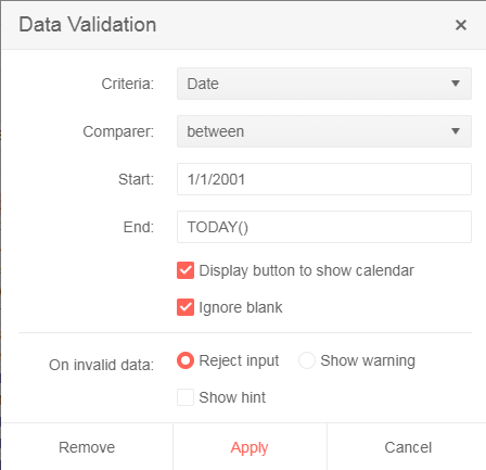
There is an issue with the Date type fields validation in the Spreadsheet. 

Here are the reproduction steps:

1. Open https://demos.telerik.com/kendo-ui/spreadsheet/index

2. Import attached xlsx file.

3. There are two date cells (B1 & B2), B2 has a data validation (Date between B1 to ToDay)

4. Try to edit the date using the calendar icon from B2. An empty calendar appears

Note: If I change data validation (remove reference of B1 and put hardcoded date) as below then it works.

Expose API that would allow a check of whether filtering has been applied to a given range/sheet. Especially identify the case when filtering is applied but no items were filtered out.

For the time being the Spreadsheet parser is unable to read files which tags are not in the default namespace. Try to open the attached file in this demo project: https://demos.telerik.com/kendo-ui/spreadsheet/index. 

You won't be able to load the file. If you open the file in Excel, save the file ("Ctrl+S") and try to load it in the Spreadsheet again, there will be no issues with it. The difference in file's structure before and after being saved in Excel could be seen in the attached screenshot.

The code in red is the structure of the file before saving it and the one in green is after the "save" operation. The difference between the files is that the structure of the one saved in Excel inserts the tags in the default namespace while the original document uses the "x:" namespace. 

It will be very useful if we can load files with defined namespaces in their structure. 

Bug report

The Spreadsheet doesn't' load correctly Excel files which definition of the tag is a single cell, instead of a cell range.

Test files: test-2.zip

Reproduction of the problem

1. Download the test-2.zip file and load the "test.xlsx" file in the Spreadsheet here.
2. The file has data in the “AZ” and “BA” columns and once it is imported in the Spreadsheet the data from the “BA” column is imported in the “AX” column and the values in the AZ column are missing.

• If the above file is saved in Excel it is correctly loading in the Spreadsheet. In the attached archive there is the “test-copy.xlsx” file which is the saved and correctly working one. Below is the structure of the two files. The one in red is from the "test.xlsx" file and the code in green is from the "test-copy.xlsx" file.

Current behavior

The The "test.xlsx" file is not loading correctly in the Spreadsheet and loses data

Expected/desired behavior

The "test.xlsx" file should load correctly in the Spreadsheet without losing data

Environment

• Kendo UI version: 2020.1.219
• jQuery version: x.y
• Browser: [all]

Dear Concerned,

1. open https://demos.telerik.com/kendo-ui/spreadsheet/index

2. select row header of row 10, go to Insert tab

3. click insert row below, it inserts row successfully after row 10, it adjust formulas of row 12, and other rows there after which is good.

4. But issue is - it neither keep format of row 10 in new row & nor it add formulas to various columns in new row(e.g. F11, E11)

Please suggest how can we achieve it, it is very common and useful feature which excel have. if you do not have any ready solution then please suggest workaround for the same as it is urgent for my client.

Need:

Extract only the values for all Spreadsheet cells. These extracted values can be sent back to server (with minimum size) as server only needs data on each sheet. On other information required like references, formulas, images, colors etc.

 

Possible Approach:

On click of save or a separate button, which will generate a low size data file (having sheet name, cell index and value), which we can send to server.

 

It will save network traffic and also no complex parsing needed at server side to fetch data.

 

Bug report

The AND formula, when used as part of an array formula, does not evaluate the whole array.

{=AND(A1:D1="")} would return TRUE if a value is entered in the range B1:D1 and FALSE only if value is entered in A1
=IF(AND(A1="",B1="",C1="",D1=""),TRUE,FALSE) would return FALSE if value is entered in any cell in range A1:D1

Reproduction of the problem

1. Run this dojo
2. Select cell E1, press F2 to edit formula and press Ctrl+Shift+Enter to enter as an array formula

Current behavior

1. Enter a value in cell B1 - Array formula evaluates as TRUE, Non-array formula as FALSE
2. Only if a value is entered in A1 the Array formula will evaluate as FALSE

Expected/desired behavior

Array formula should be evaluated correctly and return FALSE when a value is entered in any cell in range A1:D1.

Environment

• Kendo UI version: 2020.2.617
• Browser: [all]

Bug report

Reproduction of the problem

Use the Events demo to reproduce, since the events are logged in the console: https://demos.telerik.com/kendo-ui/spreadsheet/events

1. Add a new sheet
2. Drag left the newly added sheet, to make it first
3. Click "Invoice", hold down the mouse button and drag the Invoice sheet back to first place

Current behavior

The Invoice sheet is selected but the selectSheet event does not fire.

Expected/desired behavior

The selectSheet event fires

Environment

• Kendo UI version: 2020.2.617
• jQuery version: x.y
• Browser: [all]

Since the Spreadsheet does not support macros, implement error handling in the widget that notifies the user if they attempt to load a file that contains a macro. For more details see: Ticket ID: 1486172