Bug report
When the Spreadsheet is bound to a DataSource upon making multiple selections in the Spreadsheet and deleting the selected ranges a JavaScript error is thrown: "Unsupported for multiple ranges." The selected cells are deleted on the UI, but the DataSource change event is not triggered.
Reproduction of the problem
- Run the demo on DataSource binding
- Make random multiple selections
- Delete selection using the Delete key
Current behavior
A JavaScript error is thrown: "Unsupported for multiple ranges." The selected cells are deleted on the UI, but the DataSource change event is not triggered.
Expected/desired behavior
Upon an attempt to delete multiple selections a popup should be displayed with a warning that this operation is not supported, similar to trying Copy/Paste multiple selections.
Environment
- Kendo UI version: 2020.1.219
- Browser: [all]
API Reference - https://docs.telerik.com/kendo-ui/api/javascript/spreadsheet/range/methods/bold
Response to the dropped question - https://www.telerik.com/forums/spreadsheet#oqgnX2WUgkamRHjKylHvlg
This is observed also in online demos:
Steps:
- Open demo
- Edit a cell and enter text
- Press Alt+Enter and enter more text
- Press Alt+Enter
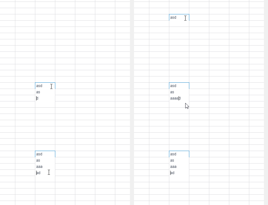
Result: the last letter of the row is transferred to the new row
For the time being the Spreadsheet parser is unable to read files which tags are not in the default namespace. Try to open the attached file in this demo project: https://demos.telerik.com/kendo-ui/spreadsheet/index.
You won't be able to load the file. If you open the file in Excel, save the file ("Ctrl+S") and try to load it in the Spreadsheet again, there will be no issues with it. The difference in file's structure before and after being saved in Excel could be seen in the attached screenshot.
The code in red is the structure of the file before saving it and the one in green is after the "save" operation. The difference between the files is that the structure of the one saved in Excel inserts the tags in the default namespace while the original document uses the "x:" namespace.
It will be very useful if we can load files with defined namespaces in their structure.
1. Open https://demos.telerik.com/kendo-ui/spreadsheet/index
2. Move horizontal scroller to column P
3. Now select Row 1 header, then row 2 header and keep doing it
4. Please observe horizontal scroller is also moving towards left
I assume it is a bug and need a fix. Meanwhile if you can provide a workaround for the same if possible.
Note: Similar behavior can be noted for vertical scroller on column header selection
Dear Concerned,
1. Open https://demos.telerik.com/kendo-ui/spreadsheet/index
2. Select column B and drag mouse towards C, both columns will be selected which is correct behavior
3. Now just scroll down 2-3 rows using vertical scroll bar
4. Repeat step 2, this time it does not select B & C, instead it selects B,C,D,E.
5. Seems a bug, not an expected behavior.
Observation that might help you in fixing it:
1. if you move scroll bar in such a way so that no merged cell is visible it works well, e.g. scroll down till 20th row becomes first visible row on screen and now repeat step 2, it will work
2. if scroll position is on top then behavior is correct as well
3. Same issue exists in case of multiple row selection with merged column and scroll position.
There is an issue with the Date type fields validation in the Spreadsheet.
Here are the reproduction steps:
1. Open https://demos.telerik.com/kendo-ui/spreadsheet/index
2. Import attached xlsx file.
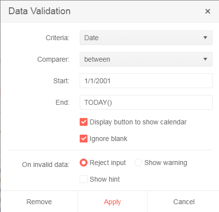
3. There are two date cells (B1 & B2), B2 has a data validation (Date between B1 to ToDay)
4. Try to edit the date using the calendar icon from B2. An empty calendar appears
Note: If I change data validation (remove reference of B1 and put hardcoded date) as below then it works.
Bug report
If an Excel file that contains Shapes is imported in the Spreadsheet, the imported content cannot be exported back to '.xlsx' file. Saving the imported content to Excel throws an error in the console.
Reproduction of the problem
- Open this demo
- Import the attached "Download Issue.xlsx" file that has one shape and one Image in the Sheet1.
- The file import will be successfully executed. The shape from the file is not visible in the Spreadsheet(this is expected behavior as the Spreadsheet component does not support Shapes, so they are ignored during the import process)
- Export(save) the Spreadsheet content as Excel file
Current behavior
Exporting the Spreadsheet content throws an error in the console:

Expected/desired behavior
The Spreadsheet content should be exported to Excel file that doesn't contain the shapes from the imported file
Environment
- Kendo UI version: 2019.3.1023
- jQuery version: x.y
- Browser: [all]
Bug report
Reproduction of the problem
Dojo example.
Current behavior
The first row is duplicated.
Expected/desired behavior
The first row is not duplicated
Environment
- Kendo UI version: 2019.3.1023
- jQuery version: x.y
- Browser: [all]
Hello,
Is is possible to trigger validation in cells in spreadsheet control? I want to make all validation controls with a button click outside the spreadsheet control.
Bug report
Office 365 Comment are shown with a warning:
"[Threaded comment]
Your version of Excel allows you to read this threaded comment; however, any edits to it will get removed if the file is opened in a newer version of Excel. Learn more: https://go.microsoft.com/fwlink/?linkid=870924
Reproduction of the problem
go to demo - https://demos.telerik.com/kendo-ui/spreadsheet/index
Current behavior
import a file from ticket - 1447268
A warning is displayed
Expected/desired behavior
No warning is displayed
Environment
- **Kendo UI version: 2019.3.1023
Bug report
There is no TypeScript definition for defineFunction and no custom functions can be created in TypeScript context using the approach demonstrated in this Custom functions article.
Reproduction of the problem
Try defining a new function using:
kendo.spreadsheet.defineFunction("Mask",mask).args(maskArgs)
Current behavior
The following error appears:
Propery "defineFunction" does not exist on type 'typeof spreadsheet'
Expected/desired behavior
There shouldn't be any errors
Environment
- Kendo UI version: 2019.3.1023
- jQuery version: x.y
- Browser: [all]
1. Open https://demos.telerik.com/kendo-ui/spreadsheet/index
2. Put some text in B2 so that it does not fit in the cell width.
3. Press Wrap Text button
4. Press Wrap Text again
5. The row height is not adjusted back to the original height (Excel does it)
1. Open https://demos.telerik.com/kendo-ui/spreadsheet/index
2. Import attached Book1.xlsx. Observe Cell F4 of Sheet1 has a font size of 72.
3. Change it to 8, row height does not change automatically
4. It should be same as Excel behavior
Please provide a fix or any workaround in the meanwhile.
https://demos.telerik.com/kendo-ui/spreadsheet/index
1. Enter some text in a cell.
2. Increase the cell font size to 48.
3. Reduce the cell font size to 8.
4. Double click the row resize handler: the row height is not adjusted to correspond to font size 8.
The same behavior can be observed when opening an existing .xlsx file that has some text and font size set and following steps 3-4.
Hi,
I encountered a bug when using the spreadsheet control with a remote datasource which I was able to replicate using the datasource binding demo (https://demos.telerik.com/kendo-ui/spreadsheet/datasource).
When entering data on an empty cell in an empty row not adjacent to a non-empty row (e.g. a row that is two rows below the end of the data); then editing a cell in the same row, but adjacent column, this creates two items in the corresponding datasource.
Editing an empty row above this new row will modify one of the records created in this process.
It would be very useful if Kendo can provide two more functions like fromJSON & toJSON in a Spreadsheet as mentioned below
fromStream() - to load an excel file form an Excel stream string so that the developer does not need to convert it to blob etc.
toStream() - to return excel stream string, it would good if it is possible to get stream without blocking UI operation. As of now, we first call toJSON & then call kendo.ooxml.Workbook(jsonSpreadsheetData).toDataURL(); to get excel stream and it is time consuming operation.
Use case: keeping excel file/stream on the server and fetching it using API on UI and then using fromStream to load & render it. And toStream is the same as toJSON to save modified stream back to the server since stream size is very low as compared to json.
Please see if it is feasible to provide these features.
Dear Concerned,
1. Open https://demos.telerik.com/kendo-ui/spreadsheet/index
2. Import attached Book21.xlsx file
3. I have first row as frozen pane and columns C, D are hidden
4. Select columns B to E using mouse drag & then right click on selected column , it does not show Unhide option, because on right click it keeps the selection only on column E
It does not work if we keep Freeze Panes.


