Currently, when trying to load a corrupt XLSX file, the Spreadsheet will freeze and no message will be returned to the user. Improve the widget to unfreeze the view and notify the user about the problem.

Add option for manual calculation of formulas, as available in Excel.

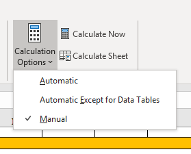
It would be a great feature to have to save time for inputting values without updating other dependent cells and once data entry is done user could press "Calculate Now" and all of the cells updated in one go, same as we do have this feature in MS Excel 365.

Excel supports deselecting cells from selected ranges, e.g. selecting a range from cell A1 to A10 results in a range A1:A10. Then deselecting cell A5 from that range produces two new ranges - A1:A4 and A6:A10.

Now a more complex example - selecting multiple ranges with intersecting cells - A1:B10, A5:D10, A9:C14 and A9:G9.


Deselecting cell B9 in Excel produces a new range with cell A9 only and then a range C9:G9. And B9 should be excluded from the other 3 ranges.

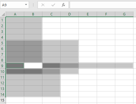
Currently the Spreadsheet widget does not know how to do this. There is no logic to decide what new ranges should be created on such operation. What it currently knows is creating new ranges and these ranges may overlap. Thus clicking on cell B9 creates a new range with cell B9, instead of deselecting B9 from the already selected ranges.

Consider implementing functionality for importing and working with encrypted / password protected Excel files in the SpreadSheet component

Enhancement

Please refer to this Dojo example - https://dojo.telerik.com/IRIRahoS/2.

Current behavior

Currently, if the filter configuration is not explicitly set, the filter button from the toolbar seem inefficient. If you toggle a filter for a column, that filter is applied for that column only. In Excel, the filter will be applied for all columns. Also, you need to manually select all the cells that you wish to filter/sort.

Steps to observe the above:
In the Dojo example, toggle filter for a column only (without manually selecting cells).

You can see that the filter will be applied for that column only. Please compare to Excel.

You will see that there is no content to be filtered/sorted. You need to select manually. Again, please compare to Excel.

Expected/desired behavior

When the filter button is pressed, execute the filter configuration logic, so that it will behave as Excel.
filter: { ref: "A3:G49", columns:[] },

Currently, the Spreadsheet component doesn't have the functionality to create a formula using the keyboard arrows.

For example:

1. Open: https://demos.telerik.com/kendo-ui/spreadsheet/index 

2. Select C12 and type =SUM( to set formula 

3. Use the arrow keys to select the starting cell. This functionality is not available.

Please provide the described above functionality.

Hi

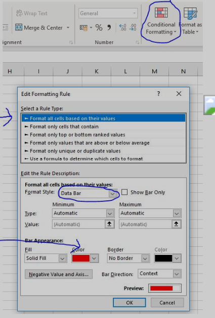
Does the kendo spreadsheet support conditional formatting / data bars (which are the background bar charts on a cell)...

See example below - and attached simple xlsx (in zip)

 

which in excel you add like

 

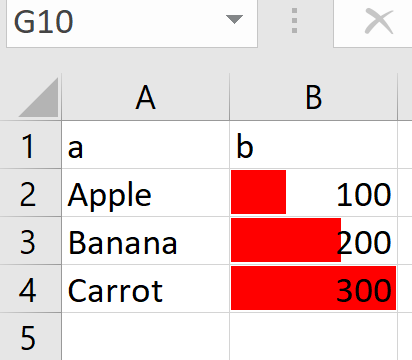
If not currently supported as standard, any suggested workarounds?

Thanks

 

Chris

The filtering on the spreadsheet component is great!!

There is however one behaviour that causes confusion for end users, and that is filtering when merged cells  are present in the selection.  
An example is available in the following dojo:
https://dojo.telerik.com/UzUMUDos

Open the dojo and filter column A on a1 and you will only see only b1 in column B, but the b1a will not be shown.

To be clear - This is also how Excel behaves...  (which is of course your prime aim so its not a bug as such)... 
Interestingly google sheets stops you putting filter on merged cells / stops you merging on filtered column.

The Excel behavior is discussed in the following threads:
https://stackoverflow.com/questions/49816515/excel-filtering-for-merged-cells
https://www.officetooltips.com/excel_2013/tips/workaround_for_sorting_and_filtering_of_merged_cells.html

Is it possible to implement something, so the end user experience would be improved? Maybe when merged cells are present :
a) if they click filter, this is detect and user is warned of this behaviour
b) if they click filter, the sheet is changed into an unmerged version (which repeats data in merged cells) as in the excel examples above.

 

Currently the API does not provide a way to detect when filtering occurs. It would be great if you could add a filter event.

I need some event which gets fired when cell data validation gets failed, with entered what value got entered by the user and cell row and column index.

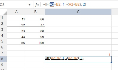
We have a client that recently brought to our attention the fact that he found a case where he couldn't place his cursor in a certain spot of a formula, click a cell, and have it fill that cell in. It works if you try to do that for the first cell listed in the formula, but not the rest. I've outlined a sample case below.

You can enter a formula in a cell like =IF(A2+B2, 1, -(A2+B2), 2). Then, highlight a cell, like A2 below, and delete it by hitting backspace or delete.

After hitting delete, leave the cursor in the same location of the formula and click a new cell, like A4.

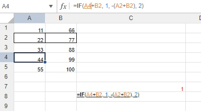
For this case, since it's the first cell in the formula, it will insert the cell you just clicked on in the correct location. However, next try highlighting the next cell referenced, hitting delete, and clicking on a new cell to have it insert the cell into the formula. In this case, we highlighted and deleted B2, then tried to click on B4.

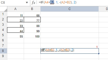
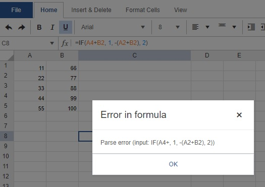
You'll see that, for this one, instead of inserting B4, it gives an error message. Our client said that it significantly slows him down when he has to manually type in each change to the formula, so is there any way we could have it insert the cell you click on for all cases? It doesn't look like this is a current feature, so would you be able to add it, please? Thank you!

Bug report

Reproduction of the problem

Reproducible in the demos.

1. Use the HYPERLINK function in a cell:

=HYPERLINK("https://google.com")

Current behavior

The link does not work. It does if you specify a "friendly name":
=HYPERLINK("https://google.com", "google")

Expected/desired behavior

The link works with and without a "friendly name" specified, as in Excel.

Environment

• Kendo UI version: 2019.2.619
• jQuery version: x.y
• Browser: [all]

Currently there is no suitable event to detect cell styling changes. Such event could be implemented similar to the formatChange event but for the styling changes.

Dear Concerned,

1. Launch https://demos.telerik.com/kendo-ui/spreadsheet/index

2. Import attached Dummy.xlsx file

3. No data loaded

4. please check

 

 

Other spreadsheet applications (Excel and Google Sheets, to name two) offer the ability to insert individual cells into a sheet without inserting a whole row/column. Most importantly, this feature updates cell references in formulas, which is not something that can be done with copy and paste.

For example, in the following spreadsheet (screenshot from Excel), I've right-clicked cell A2 and chosen "Insert" on the context menu. There is also a button on the ribbon that opens the same "Insert" dialog.

I want to shift the cells down, so I click OK in the dialog. Note that the formulas update accordingly: the sum range expands to A1:A5, while the individual cell references remap.

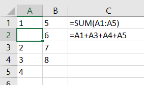
Can this feature please be added to Kendo spreadsheet? Otherwise, our clients will have to continue manually re-writing formulas after they copy/cut and paste to achieve a similiar-looking (but functionally different) result.

Thanks!

 

Dear Concerned,

 

1. Launch https://demos.telerik.com/kendo-ui/spreadsheet/index

2. Open Attached Test.xlsx file

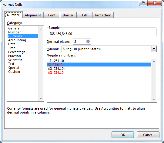
3. Check the value of A2, it is different than Excel

Note: Cell format of A2 is set as below, if I select only $ format then it is working.

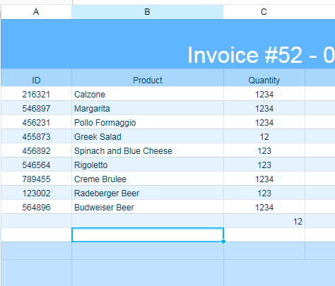
On Internet Explorer-11, UI is getting blocked while performing comparatively fast data entries, it is not only too slow but values are getting truncated as well.

 

1. Open https://demos.telerik.com/kendo-ui/spreadsheet/index in IE 11

2. Start editing cells C3 to C12 and enter value 1234 in each cell as fast as possible

3. 1234 enter, 1234 enter , 1234 enter and so on without waiting for UI rendering completion as UI freezes for few seconds, and then all cells get updated in one go

4. below is the result, few cells are having wrong values 

5. Its very serious issue

Note: Excel 365, Excel and GoogleSheet works fine in such cases

Hi again :)

I see that in the configuration I can specify the max number of rows/column. However, I can do it per component basis, and I would like to have that on a per-sheet basis. Any way I can implement this?

Thanks!

Provide support for images client-side import/export through Telerik Document Processing.

Wanting to format a subset of a single cell with text styling different from the rest of the cell contents.  Something like the following:

or