Ability to set a cell with font Strikethrough
For the time being the Spreadsheet parser is unable to read files which tags are not in the default namespace. Try to open the attached file in this demo project: https://demos.telerik.com/kendo-ui/spreadsheet/index.
You won't be able to load the file. If you open the file in Excel, save the file ("Ctrl+S") and try to load it in the Spreadsheet again, there will be no issues with it. The difference in file's structure before and after being saved in Excel could be seen in the attached screenshot.
The code in red is the structure of the file before saving it and the one in green is after the "save" operation. The difference between the files is that the structure of the one saved in Excel inserts the tags in the default namespace while the original document uses the "x:" namespace.
It will be very useful if we can load files with defined namespaces in their structure.
Currently the spreadsheet dynamically creates the FilterMenu for a range, that is, it's not created until someone clicks the filter dropdown, and it's destroyed if they switched tabs.

There is no event that is fired when these things happen, which makes it hard to attach to, and customize, the FilterMenu without setting up some crazy listening code (setTimeout, etc.).

It would be great if either (or both:
- You could specify a template for the filter menu.
- You could listen for a "FilterMenu Initialized" event and capture the menu there and customize it.
Dear Concerned,
1. Open https://demos.telerik.com/kendo-ui/spreadsheet/index
2. Select column B and drag mouse towards C, both columns will be selected which is correct behavior
3. Now just scroll down 2-3 rows using vertical scroll bar
4. Repeat step 2, this time it does not select B & C, instead it selects B,C,D,E.
5. Seems a bug, not an expected behavior.
Observation that might help you in fixing it:
1. if you move scroll bar in such a way so that no merged cell is visible it works well, e.g. scroll down till 20th row becomes first visible row on screen and now repeat step 2, it will work
2. if scroll position is on top then behavior is correct as well
3. Same issue exists in case of multiple row selection with merged column and scroll position.
I want to be able to double click a column header to set column width to max width of entries - autoresize
Bug report
When a string, used as old_text for SUBSTITUTE(text, old_text, new_text, [instance_num]) function, is repeated more than once and the new_text is an empty string, one occurrence of the old_text remains not substituted.
Reproduction of the problem
- Go to Spreadsheet Basic usage demo
- Add a new sheet
- Type
ab113abababab11abin A1 - Enter the following formula in B1
=SUBSTITUTE(A1, "ab", "")
NOTE: substituting ab with another string, e.g. cd, replaces all instances of ab as expected.
Current behavior
113ab11 - when ab is repeated more than once in a row, one of its instances remains unchanged to an empty string
Expected/desired behavior
11311
Environment
- Kendo UI version: 2019.2.514
- Browser: all
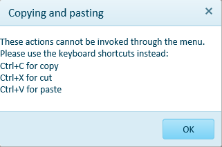
When using IE 11 and using Ctrl+X to cut, this only works the first time. All subsequent attempts to use cut produce the following dialog:
Error occurred in browser console after select cell with value, pressing cut scissors button on top and press undo shortcut key combination (Ctrl+Z at windows or Cmd+Z at macos)
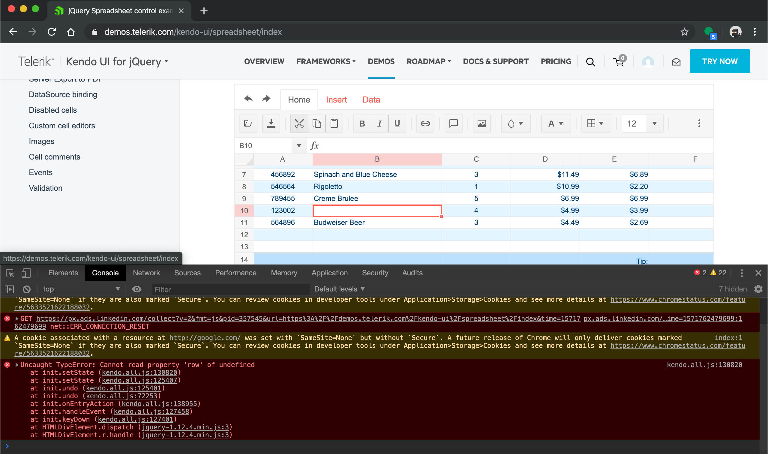
at init.setState (kendo.all.js:130820)
at init.setState (kendo.all.js:125407)
at init.undo (kendo.all.js:125401)
at init.undo (kendo.all.js:72253)
at init.onEntryAction (kendo.all.js:138955)
at init.handleEvent (kendo.all.js:127458)
at init.keyDown (kendo.all.js:127401)
at HTMLDivElement.dispatch (jquery-1.12.4.min.js:3)
at HTMLDivElement.r.handle (jquery-1.12.4.min.js:3)
setState @ kendo.all.js:130820
setState @ kendo.all.js:125407
undo @ kendo.all.js:125401
undo @ kendo.all.js:72253
onEntryAction @ kendo.all.js:138955
handleEvent @ kendo.all.js:127458
keyDown @ kendo.all.js:127401
dispatch @ jquery-1.12.4.min.js:3
r.handle @ jquery-1.12.4.min.js:3
Bug report
File:
3f0465a2-412c-4876-ba47-4b12ae46f92e_adam.zip
https://demos.telerik.com/kendo-ui/spreadsheet/index
Reproduction of the problem
- Import the file
Current behavior
Errors are encountered. Even if resolving the errors bold styles are not applied as they are part of the font definition and not of the inlineStyles.
Expected/desired behavior
The excel is imported as expected.
Environment
- Kendo UI version: 2019.2.514
- Browser: all
Bug report
The current client-side export functionality does not preserve the number of columns.
Reproduction of the problem
Load the following file in the Spreadsheet which contains columns up to "BA".
Export the file
Load the file again in the Spreadsheet and notice that the columns are displayed up to "AX" instead of "BA".
Current behavior
Client-side export does not preserve the number of columns greater than "AX".
Expected/desired behavior
Client-side export does not preserve the exact number of columns.
Environment
- Kendo UI version: 2019.2.619
- Browser: [all]
The Ctrl + Shift + Arrow key keyboard shortcut should select a range in the row/column starting with the active cell and ending with the first cell in the row/column that has a value: [list of shortcuts](https://docs.telerik.com/kendo-ui/controls/data-management/spreadsheet/end-user/list-of-shortcuts) used by the Spreadsheet. It works similarly in Excel.
### Current behavior
The selection does not end at the first cell that has a value, it ends with the last cell of the row/column.
### Expected/desired behavior
The expected behavior should be as described in the documentation: "Extends the selection of cells to the last nonblank cell in the same row or column as the active cell."
### Environment
* **Kendo UI version:** 2018.2.620
* **Browser:** [all ]
Hi Kendo Team,
The exported excel file from spreadsheet can not be opened in Microsoft excel when the spreadsheet has both a comment and a image.
You can reproduce the issue at your demo site https://demos.telerik.com/kendo-ui/spreadsheet/index
First add a comment for cell D3, then add a image, then export as xlsx.
Try open the export excel file, and you will see the error popup says "we found a problem with some content in workbook.xlsx ......"
It works when exporting comment and image separately.
Bug report
Spreadsheet SUMIF function returns #NA when Excel returns the correct result. The issue is observed when the criteria range and sum range have different sizes.
Reproduction of the problem
Run the Spreadsheet demo page
Open the attached file
Formula in cell B3 returns #NA!
Current behavior
The formula in cell B3 returns #NA!
Expected/desired behavior
The formula in cell B3 should return the correct value
Environment
Kendo UI version: 2019.3.1023
Browser: [all]
Dear Concerned,
1. Open https://demos.telerik.com/kendo-ui/spreadsheet/index
2. Import attached Book21.xlsx file
3. I have first row as frozen pane and columns C, D are hidden
4. Select columns B to E using mouse drag & then right click on selected column , it does not show Unhide option, because on right click it keeps the selection only on column E
It does not work if we keep Freeze Panes.
Please support Excel formulas copy and paste to Kendo Spreadsheet.

Now is the copy only the text, not formulas.
https://demos.telerik.com/kendo-ui/spreadsheet/index
1. Enter some text in a cell.
2. Increase the cell font size to 48.
3. Reduce the cell font size to 8.
4. Double click the row resize handler: the row height is not adjusted to correspond to font size 8.
The same behavior can be observed when opening an existing .xlsx file that has some text and font size set and following steps 3-4.
1. Open https://demos.telerik.com/kendo-ui/spreadsheet/index
2. Put some text in B2 so that it does not fit in the cell width.
3. Press Wrap Text button
4. Press Wrap Text again
5. The row height is not adjusted back to the original height (Excel does it)
1. Open https://demos.telerik.com/kendo-ui/spreadsheet/index
2. Import attached Book1.xlsx. Observe Cell F4 of Sheet1 has a font size of 72.
3. Change it to 8, row height does not change automatically
4. It should be same as Excel behavior
Please provide a fix or any workaround in the meanwhile.